
Calculating entropy production of active field theory
Published:
In this blog post we will discuss how to calculate entropy production in active field theories, taking into account of temporal discretization and Ito/Stratonovich issues.
Entropy production
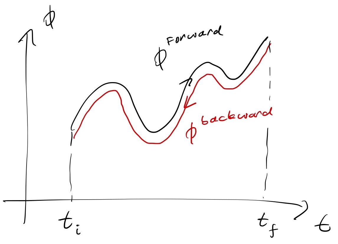
Let us consider some trajectory $\phi(\mathbf{r},t)$ from time $t = t_i$ to $t = t_f$. The rate of entropy production $\mathcal{S}$ is defined to be the logarithm of the ratio of forward probability to the backwards probability:
\[\mathcal{S} = \lim_{(t_f-t_i)\rightarrow\infty} \frac{1}{t_f-t_i} \left<\ln\left(\frac{P_F[\phi]}{P_B[\phi]}\right)\right>\]where $P_F[\phi]$ is the probability functional of obtaining a particular trajectory $\{\phi(\mathbf{r},t)|t\in[t_i,t_f]\}$ and $P_B[\phi]$ is the probability functional of obtaining the same trajectory going backwards in time (see image below). In another word, entropy production is a measure of time-irreversibility.
The angle brackets above $\left<\dots\right>$ indicates averaging over all noise realizations.
Entropy production for active model B
Active model B is a model for phase separation in active matter, which is a derivative of the active model B+ (see previous post). The active model B dynamics is given by:
\[\frac{\partial\phi}{\partial t} + \nabla\cdot\left(\mathbf{J}_{d} + \boldsymbol{\Lambda}\right) = 0\]$\mathbf{J}_d$ is the deterministic current and $\boldsymbol{\Lambda}$ is a Gaussian white noise with zero mean and delta function correlation:
\[\left<\Lambda_\alpha(\mathbf{r},t)\Lambda_\beta(\mathbf{r}',t')\right> = 2D\delta_{\alpha\beta}\delta(\mathbf{r}-\mathbf{r}')\delta(t-t')\]The deterministic current is given by:
\[\mathbf{J}_{d} = -\nabla\underbrace{\left(\frac{\delta F}{\delta\phi} + \lambda|\nabla\phi|^{2}\right)}_{\mu}\]where $\mu$ is the chemical potential, which consists of the passive/equilibrium part: $\delta F/\delta\phi$ and the active part: $\lambda|\nabla\phi|^2$ The rate of entropy production for this dynamics can be shown to be given by (Nardini, Fodor, Tjhung, van Wijland, Tailleur, Cates, PRX, (2017)):
\[\begin{align} \mathcal{S} & =\frac{1}{\tau}\int_{0}^{\tau}dt\,\frac{\partial\phi}{\partial t}\circ\mu\nonumber \\ & =\frac{1}{\tau}\sum_{t}\Delta t\frac{\phi_{t+\Delta t}-\phi_{t-\Delta t}}{2\Delta t}\mu_{t},\nonumber \end{align}\]where the time integral is interpreted as Stratonovich. $\phi_t$ is the density field at time $t$ and $\mu_t$ is the chemical potential at time $t$. The reason for the Strotonovich choice is follows:
When we are computing entropy production, basically, we are comparing the trajectory going forward in time and the trajectory going backwards in time.
Now the time is discretized into $t = 0, dt, 2dt, 3dt, \dots$. That means the trajectory is also split into segments. The way we split the trajectory is done in the Stratonovich way. That means the value of $\phi$ at time $t$ means the value of $\phi$ mid-point of $[t, t+dt]$. i.e. $\phi(\mathbf{r},t+dt/2)$. If we discretize the trajectory in `Ito’ way, the time-reversed of that trajectory is not identical (see drawing below).
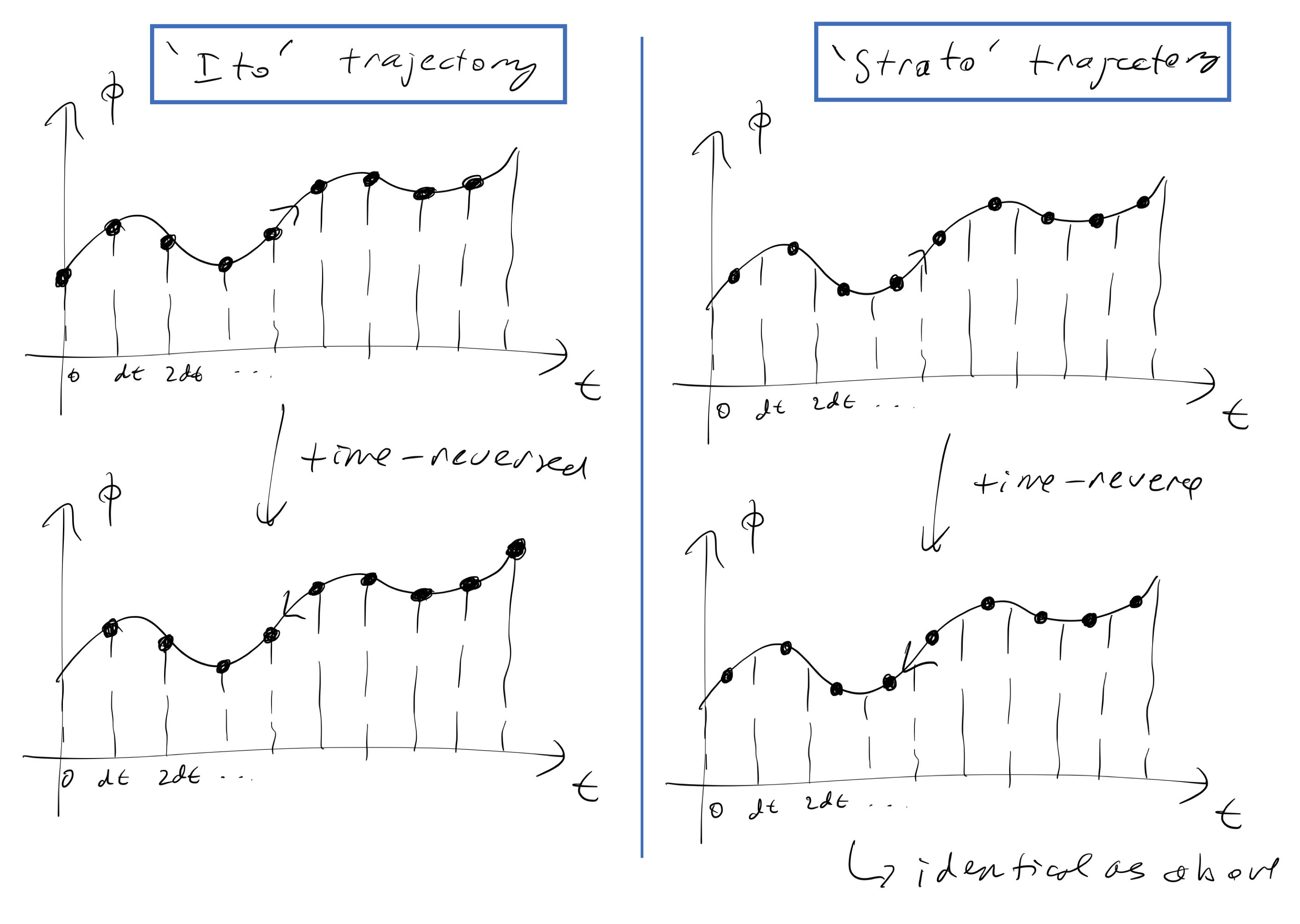
However, when we perform the simulations, we do it in `Ito’ way. i.e. we start from $\phi(\mathbf{r},0)$, then we update the time to get $\phi(\mathbf{r},0), \phi(\mathbf{r},dt), \phi(\mathbf{r},2dt), \phi(\mathbf{r},3dt), \dots$.